Tornado Chart in Excel (Easy Learning Guide)
Click on it. We have our chart but does not look good. Correct the Y-axis: Right-click on the y-axis. Click on the format axis. In labels, click on label position drop-down and select low. Now the chart looks like this. Select any bar and go to formatting. Reduce the gap width to zero and put borders as white.

Tornado Chart in Excel Step by Step tutorial & Sample File »
Create a Stacked Bar Chart by following the path Insert > Charts > Insert Column or Bar Chart > Stacked Bar Chart. Although these two steps are enough to create a basic tornado chart. Consider a few tweaking steps to polish your chart. Start by changing or removing the title according to your needs.
How to Create a TORNADO CHART in Excel (Sensitivity Analysis)
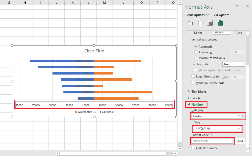
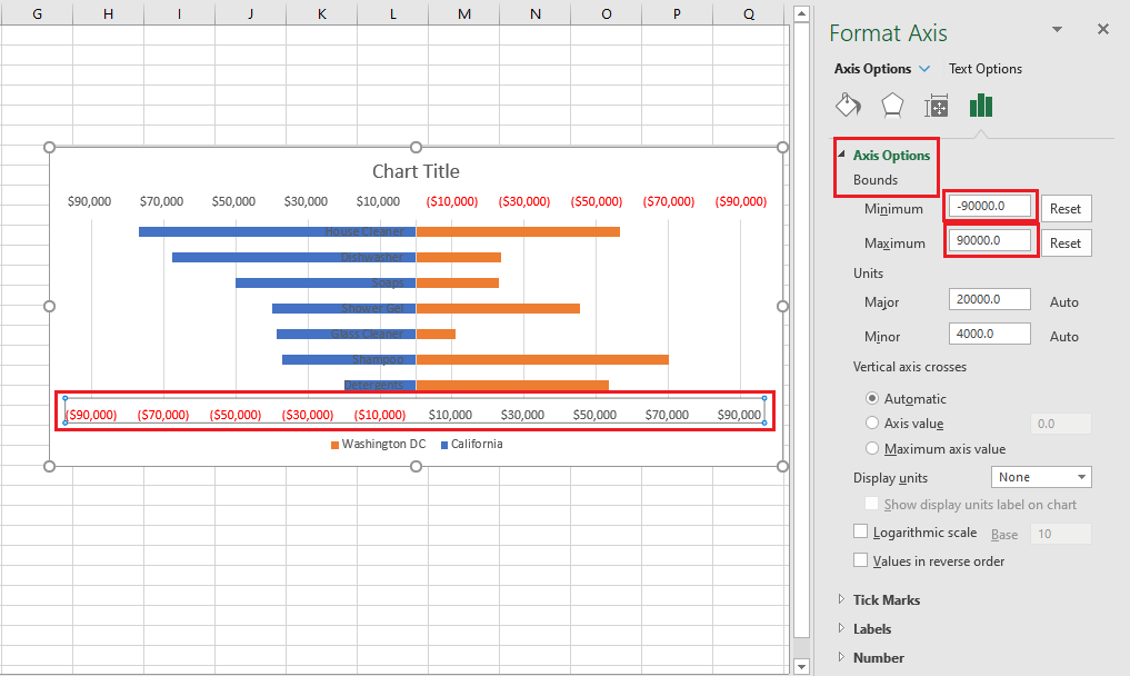
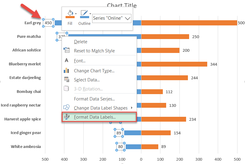
This is how our tornado gets in shape by now:-. Set the Number Format of Secondary Axis Labels as #;# and then delete the gridlines and primary horizontal axis by selecting and pressing the delete key. Format the Bars on the chart and add Data Labels. Set the position of labels at the inside end to get this:-.
Tornado Chart Excel Template Free Download How to Create Automate Excel
Understanding the data Before creating a tornado chart in Excel, it is important to understand the data that will be used to construct the chart. This involves selecting the appropriate data and identifying the primary and secondary variables for the chart. A. Select the data to be used in the tornado chart
How to Create a TORNADO CHART in Excel (Sensitivity Analysis)
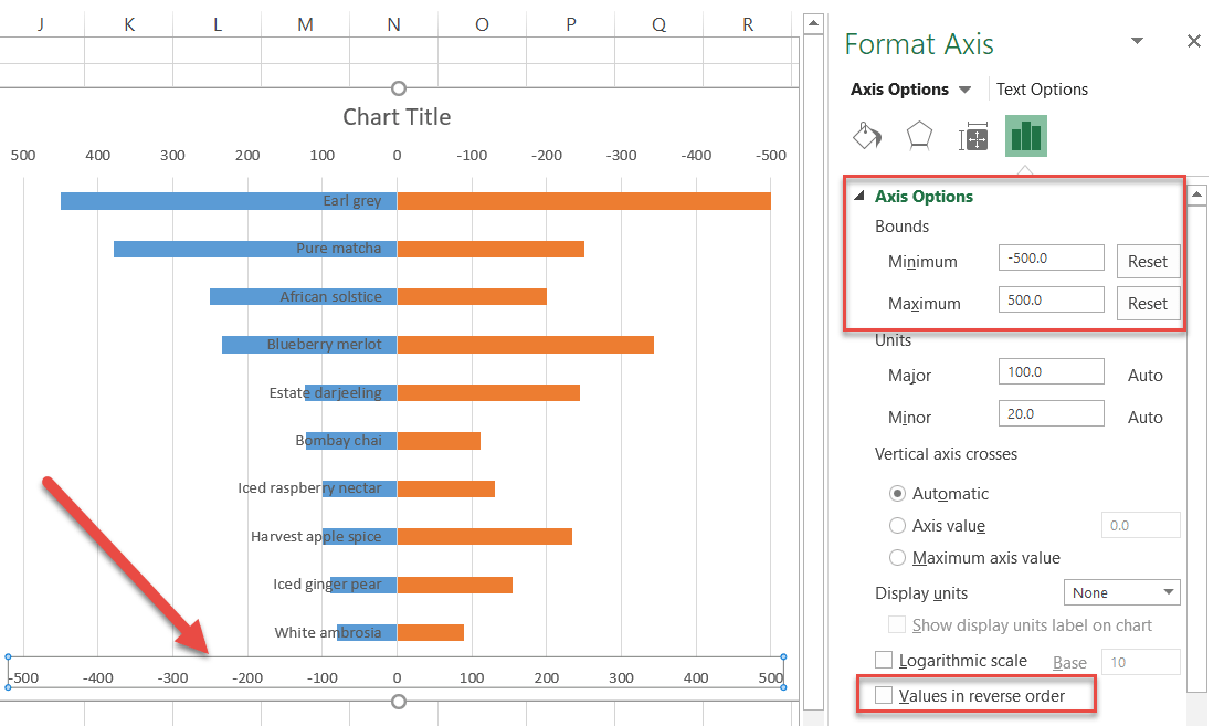
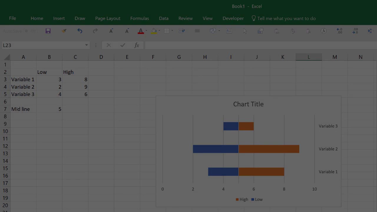
1. Prepare the data To center the chart, add the negative symbol (the symbol minus "-") to all values of the data series you prefer to see on the left (see how to quickly transform your data without using formulas ). 2. Create a simple bar chart 2.1. Select the data range (in this example, B2:D8 ). 2.2.

Tornado Chart in Excel Step by Step tutorial & Sample File »
Use a stacked bar graph to make a tornado chart.Make sure you have two columns of data set up for the tornado chart.1. We'll need one of the columns of data.
How to Create a TORNADO CHART in Excel (Sensitivity Analysis)
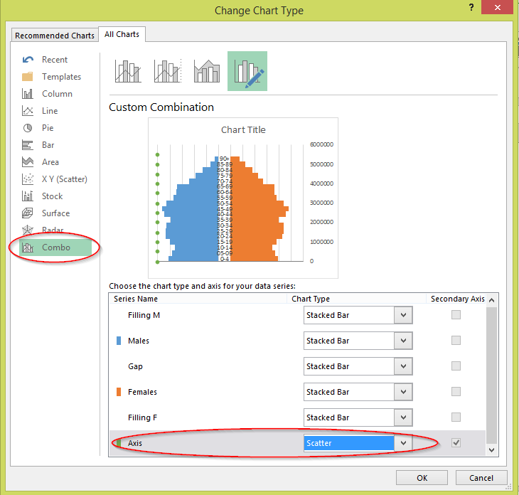
Select the XLSTAT/ Visualizing data / Tornado diagram. The dialog box pops up. In the XLSTAT interface, select tornado diagram in the format. Select the two data columns corresponding to the online and the in-store tea sales. Select the first column of the dataset as the labels. Click on OK. Interpret the Results of the Tornado Diagram

How to make a Tornado Chart in Excel YouTube
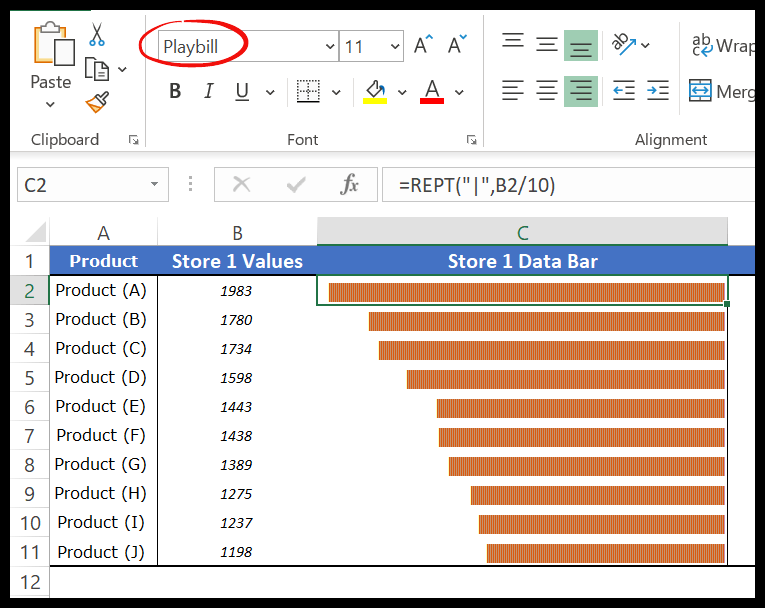
The Tornado Chart in Excel helps us graphically represent data and display the comparison as a Tornado, Butterfly, or Funnel. The Conditional Formatting and the REPT function create an in-cell Excel Tornado Chart. Independent variables cannot be used in forming a Tornado Chart, also, two variables are mandatory to show the comparison.
Tornado Chart in Excel (Easy Learning Guide)
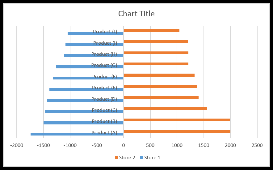
A tornado chart (also known as a butterfly or funnel chart) is a modified version of a bar chart where the data categories are displayed vertically and are ordered in a way that visually resembles a tornado.
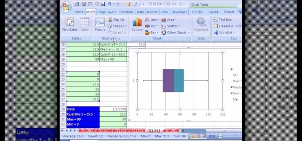
Tornado Diagram Box Plot In Excel Box Information Center
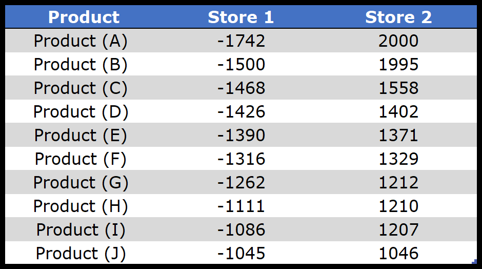
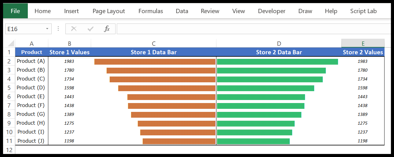
To create a tornado chart in Excel you need to follow the below steps: First of all, you need to convert data of Store-1 into the negative value. This will help you to show data bars in different directions. For this, simply multiply it with -1 (check out this smart paste special trick, I can bet you'll love it).
Howto Make a Horizontal Tornado Chart in Excel for Your Dashboard Template YouTube
Create a basic Tornado Chart in Excel 2016. Useful in showing sensitivities either deterministic or probabilistic. See my other video on Probabilistic Torn.
Tornado Chart in Excel (Easy Learning Guide)
Select a bar, right click and select Format Data Series (or press CTRL+1 for the shortcut) Under the Series Options, adjust the Series Overlap setting to 100% To make the chart easier to read, you can add Data Labels to the left and right bar charts and adjust the colors as needed Full Example
Creating a Tornado Chart in Excel 2016 YouTube
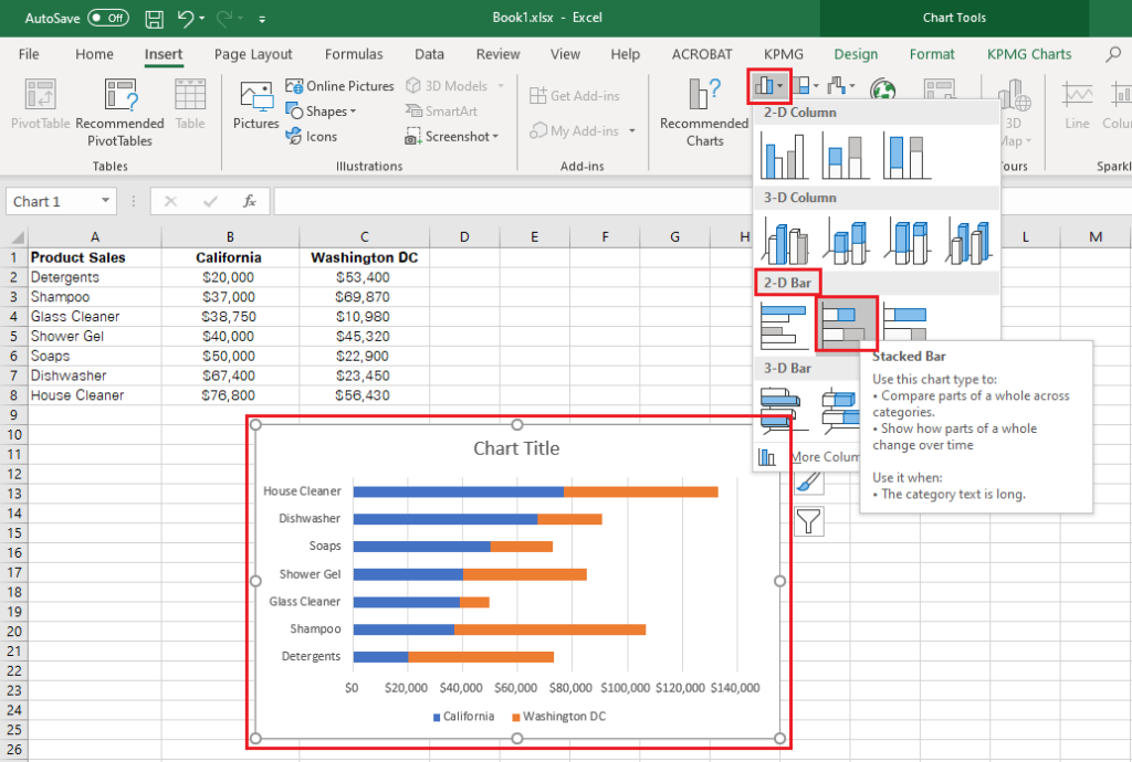
1. Selecting the data Highlight the range of data that you want to include in the tornado chart. This should typically include the variable names and their corresponding values. 2. Inserting a bar chart Go to the 'Insert' tab and select 'Bar Chart' from the 'Charts' section.
The wizard of Excel How to build a Tornado chart in Excel
A Tornado Chart is a visualization you can use to compare two contrasting variables in your data. It has two contrasting colors to show the differences in the metrics under investigation. Data visualization experts use the chart to depict the sensitivity of a result to changes in key variables.
How to Create a TORNADO CHART in Excel (Sensitivity Analysis)
Unlike other simple charts, there exists no option to create a Tornado Chart in Excel. Users, therefore, need to create a default bar chart and customize it to a tornado chart. Follow the steps below to learn how. Step 1: Below is a dataset that contains two variables i.e. sales of the same product in two different regions.
Tornado Chart Excel Template Free Download How to Create Automate Excel
How To Create a Tornado Chart In Excel? Read Jobs Tornado charts are a special type of Bar Charts. They are used for comparing different types of data using horizontal side-by-side bar graphs. They are arranged in decreasing order with the longest graph placed on top. This makes it look like a 2-D tornado and hence the name.
